
< Previous lab day | Module 2 lab index | Next lab day >
Introduction
Last time you transformed your mutant DNA into BL21(DE3) cells. The colonies that arose were moved to liquid cultures, and today you will add IPTG to these cultures to induce protein expression by the bacteria. Next time you will purify the resultant protein. I won't shy away from telling you that there are many things that can go wrong at this stage! However, each one is certainly a learning experience.
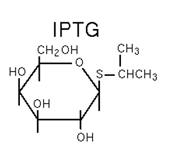
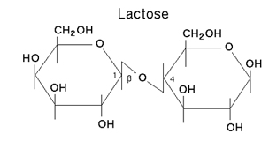
IPTG and Lactose. (Images: public domain.)
As evidenced by Nagai's work, wild-type inverse pericam is not toxic to BL21(DE3) cells. Although it is unlikely for your small mutation to dramatically change this fact, in general a novel protein may turn out to be toxic. If this is the case, only very small amounts of protein are produced before the bacteria die. Keep in mind that overexpressing a single protein may come at the expense of producing proteins needed for survival, and will most likely cause cell death eventually; however, toxic proteins hasten this demise. Aberrant toxicity can sometimes be alleviated by reducing the culture temperature (e.g., to 30 °C).
Based on its fluorescence activity, wild-type inverse pericam allows proper folding of (cp) EYFP, and based on its response to calcium, it also allows calmodulin to fold. One problem you may encounter is that your mutant proteins will no longer fold correctly. Since you made mutations in the calcium sensor part of IPC, rather than the fluorescent part, it is unlikely that your protein will destroy EYFP fluorescence. However, a common problem with misfolded proteins is the formation of insoluble aggregates, due for instance to improperly exposed hydrophobic surfaces. Proteins can be purified from these aggregates – called inclusion bodies – but the process is more labour-intensive than for soluble proteins. (The proteins must be extracted under more harsh conditions than you will use next time, then purified under denaturing conditions, before finally attempting to renature the proteins.) Inclusion bodies sometimes form simply due to very high expression of the protein of interest, causing it to pass its solubility limit. This outcome can be prevented by lowering the culture temperature or time, the amount of IPTG, or the growth phase of the bacteria.
One final point to keep in mind is that not all proteins can be produced in bacteria. Eukaryotic proteins that require post-translational modifications (such as glycosylation) for activity require eukaryotic hosts (such as yeast, or the ubiquitous CHO – Chinese hamster ovary – cells). Sometimes eukaryote-derived proteins will be truncated or otherwise mistranslated by E. coli due to differential codon bias (Kane, 1995); errors in translation can be prevented by providing additional tRNAs to the culture or directly to the bacteria via plasmids (McNulty, et al., 2003). Despite all this complexity, prokaryotic hosts have been plenty good enough to produce proteins for certain therapies, notably the cytokine G-CSF for patients needing to replenish their white blood cells (e.g., after chemotherapy), sold as Neupogen® by Amgen.
After you induce your cells with IPTG, you will let the resultant protein factories do their work for 2-3 hours. During this time, you will evaluate the DNA from your two X#Z candidates (and from the M124S mutant). First, you will run your diagnostic digests from last time out on a gel. The banding patterns will allow you to determine (or diagnose) whether either of your putative X#Z mutants actually contains the new restriction site that you introduced. Of course, there is a slim possibility that the silent mutation was incorporated but the non-silent mutation wasn't. To get more direct evidence for whether the site-directed mutagenesis worked, you will analyze data from the sequencing reactions that you set up last time.
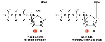
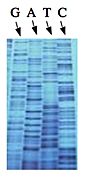
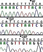
Left: Normal bases versus chain-terminating bases. Center: Sequencing gel example. Right: Sequence trace data example.
The invention of automated sequencing machines has made sequence determination a relatively fast and inexpensive endeavor. The method for sequencing DNA is not new but automation of the process is recent, developed in conjunction with the massive genome sequencing efforts of the 1990s. At the heart of sequencing reactions is chemistry worked out by Fred Sanger in the 1970s which uses dideoxynucleotides (see schematic above left). These chain-terminating bases can be added to a growing chain of DNA but cannot be further extended. Performing four reactions, each with a different chain-terminating base, generates fragments of different lengths ending at G, A, T, or C. The fragments, once separated by size, reflect the DNA's sequence. In the "old days" (all of 10 years ago!) radioactive material was incorporated into the elongating DNA fragments so they could be visualized on X-ray film (image above center). More recently fluorescent dyes, one color linked to each dideoxy-base, have been used instead. The four colored fragments can be passed through capillaries to a computer that can read the output and trace the color intensities detected (image above right). Your sample was sequenced in this way on an ABI 3730 DNA Analyzer.
Analysis of sequence data is no small task. "Sequence gazing" can swallow hours of time with little or no results. There are also many web-based programs to decipher patterns. The nucleotide or its translated protein can be examined in this way. Thanks to the genome sequence information that is now available, a new verb, "to BLAST," has been coined to describe the comparison of your own sequence to sequences from other organisms. BLAST is an acronym for Basic Local Alignment Search Tool, and can be accessed through the National Center for Biotechnology Information (NCBI) home page.
You might be wondering why you would ever go through the trouble of designing and performing diagnostic digests, when sequencing is relatively simple and yields more information. Here, the idea of scale becomes important. Sequencing costs $8 per reaction, which can add up if you need to examine, say, 10 or more candidates. Agarose gel electrophoresis, by comparison, costs perhaps $1 per candidate. Since both methods require DNA isolation, one is not dramatically more labour intensive than the other. (A method called colony PCR avoids this labour. Can you guess what it might entail?) Finally, banding patterns can give a quick readout of many candidate colonies compared to the time it takes for the individual sequencing analyses you will perform today. Of course, there's no reason one couldn't automate the analysis process with a bit of (computer, not DNA) code!
References
Kane, J. F. "Effects of Rare Codon Clusters on High-Level Expression of Heterologous Proteins in Escherichia coli." Curr Opin Biotechnol 6, no. 5 (October, 1995): 494-500.
McNulty, D. E., et al. "Mistranslational Errors Associated With the Rare Arginine Codon CGG in Escherichia coli." Protein Expr Purif. 27, no. 2 (Febraury, 2003): 365-74.
Protocols
Part 1: Cell Measurement and IPTG Induction
- For each mutant protein (X#Z candidates 1 and 2, M124S), you will be given a 6 mL aliquot of BL21(DE3) cells carrying the mutant plasmid; you will also receive a tube of BL21(DE3) carrying wild-type inverse pericam. These cells should be in or close to the mid-log phase of growth for good induction, just as they were for transformation. Like last time, check the OD600 values of your cells until they fall between 04.and 06. (Better to overshoot a little than undershoot.)
- Once your cells have reached the appropriate growth phase, set aside - on ice - 1.5 mL of cells from each tube as a control (no IPTG) sample. Then take an aliquot of cold IPTG (0.1 M), and add to your remaining cells at a final concentration of 1 mM. You should prepare three mutant and one wild-type tube.
- Return your tubes to the rotary shaker in the 37 °C incubator, and note down the time.
- While your IPTG-stimulated cells are producing protein, you will analyze the sequence data and digests of the plasmids they are carrying. At the end of the day, you will choose only one of your X#Z candidates to save, and give the other sample to the teaching faculty to be bleached and thrown away.
Part 2: Run Diagnostic Gel
The scheme below assumes that both Digest 1 (D1, used to analyze the M124S mutant) and Digest 2 (D2, used to analyze your X#Z mutant candidates) use only one enzyme. If you are doing double-digests and need to run single enzyme controls, hopefully you spoke to the teaching faculty about this last time. Load your samples on a 1% agarose gel in the following order, using 10 μL per ladder and 20 μL per plasmid:
| LANE | SAMPLE | DIGEST |
|---|---|---|
| 1 | IPC | uncut |
| 2 | IPC | D1 |
| 3 | M124S | D1 |
| 4 | 1 Kb marker | |
| 5 | IPC | D2 |
| 6 | X#Z-1 | D2 |
| 7 | X#Z-2 | D2 |
| 8 | 100 bp marker | (if relevant for your band sizes) |
| 9 | X#Z-1 | uncut |
| 10 | X#Z-2 | uncut |
Once all the samples are loaded, the power will be applied (100 V for 45 minutes) and the gel will be photographed. When the gel is ready, you will compare the band sizes in the photograph with the expected band sizes that you previously calculated. In the meantime, you can analyze your sequence data.
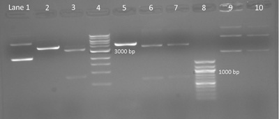
Sample gel result: Diagnostic digest testing for silent mutation on M124S, E84G, and IPC plasmids. A 1% agarose gel shows the products of a digest with AccI and BseRI on M124S, E84G, and wild-type IPC plasmid. Lane 1: IPC plasmid without restriction enzymes. Lane 2: IPC cut with AccI shows one band with linear DNA expected at 4169 bp. Lane 3: M124S cut with AccI shows two bands approximately 3331 bp and 838 bp. Lane 4: 1 kpb DNA ladder (New England BioLabs). Lane 5: IPC cut with BseRI shows linear DNA at 4169 bp. Lanes 6 and 7: E84G isolated from colony 1 and 2 respectively and cut with BseRI show two bands expected at 3515 bp and 654 bp. Lane 8: 100 bp ladder (New England BioLabs). Lanes 9 and 10: Undigested E84G, from colony 1 and 2 respectively, shows three bands. (Photo and caption courtesy of anonymous MIT student. Used with permission.)
Part 3: Analyze Sequence Data
Your goal today is to analyze the sequencing data for three samples - two independent colonies from your X#Z mutant, and one M124S clone for practice - and then decide which colony to proceed with for the X#Z mutant. You will want to have this Day 4 sequence document handy (DOC), and to mark the expected location of your mutation with bold text before proceeding. (Just compare to your annotation of the Day 1 IPC sequence document (DOC) using Word Count or the Find tool.) The new file contains the inverse pericam sequence as before, but also the flanking sequences (from the pRSET vector) before and after IPC, which are separated from IPC by a blank line. The second page of the document contains the reverse complement of IPC/pRSET, which was generated using this website tool "Reverse and/or complement DNA sequences." Be sure to bold your mutant codon in the reverse complement sequence as well.
Next we will use some data from the MIT Biopolymers Facility. [Only available to enrolled students in the class, not accessible for OCW users.] From this link, we can see sequencing traces and sequence text.
Rather than look through the sequence to magically find the relevant portion, you can align the data you just got with the standard inverse pericam sequence and the differences will be quickly identified. There are several web-based programs for aligning sequences and still more programs that can be purchased. The steps for using one web-based tool are sketched below.
Align with "bl2seq" from NCBI
- The alignment program can be accessed through the NCBI BLAST page or directly from this link.
- To allow for gaps in the sequence alignment, uncheck the "filter" box. All the other default settings should be fine.
- Paste the sequence text from your sequencing run into the "Sequence 1" box. This will now be the "query." If there were ambiguous areas of your sequencing results, these will be listed as "N" rather than "A" "T" "G" or "C" and it's fine to include Ns in the query.
- Paste the inverse pericam sequence into the "Sequence 2" box. For samples probed with the forward primer, use the regular IPC sequence; for those using a reverse primer, you should put in the reverse complement. Which alignment will be more useful depends on the location of your mutation.
- Click on Align. Matches will be shown by vertical lines between the aligned sequences. You should see a long stream of matches, followed by lots of errors in the last ~200bp of the sequence – ignore the error-ridden part of the data, as it may not accurately reflect your mutant plasmid. In this stream of matches, the 1-3 missing lines indicating your mutant codon should stand out. If they don't, use the numbering or Find tool to locate the appropriate codon.
- You should print a screenshot of each alignment to PDF (and to paper if you desire). These will be used to prepare a figure showing what you found today.
If both colonies for your mutant have the correct sequence, flip a coin and proceed with one or the other; ditto if both are inconclusive. If one appears right and the other doesn't, of course proceed with the former. Finally, if both are clearly wrong, talk to a member of the teaching faculty.
For your reference, another popular sequence alignment program is "CLUSTAL-W" from EMBL-EBI.
Part 4: Observe Mutant Colonies
Last time you transformed BL21(DE3) cells with three different plasmids (two candidates for the X#Z mutant, and one M124S clone). Compare the relative colony formation of cells carrying the different plasmids. If all the plates have dense cell growth, there is no need for you to get an exact colony count; just do your best to get a relative estimate, and describe any findings in your notebook.
Part 5: Cell Observation and Collection
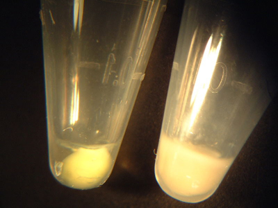
Examples of IPTG-induced (left) and control (right) cell pellets. The induced pellet has a yellow-green tint, in contrast to the plain white control pellet.
- After ~2-3 hours, you will pour 1.5 mL from each tube (from Part 1) into a labeled eppendorf, then spin for 1 min. at maximum speed. Save the other 3 mL!
- Aspirate the supernatant from each eppendorf, using a fresh yellow pipet tip on the end of the glass pipet each time.
- Observe the colour of each of your pellets, and compare to the above example. If the wild-type and both mutant pellets all appear yellow-greenish to the eye, proceed as follows:
- Do NOT toss the rest of the liquid cultures. First, measure their OD600 values, according to part 6 of today's protocol.
- Next, pour 1.5 mL more of the relevant liquid culture on top of each pellet, spin again, and aspirate the supernatant.
- The last 1.5 mL of culture may be aspirated in your vacuum flask, to be later bleached and discarded.
- If one or more of your pellets are white or only dimly coloured, please ask one of the teaching staff to show you the room temperature rotary shaker. You will continue to grow your bacteria overnight. Tomorrow morning, the teaching staff will collect your pellets for you and freeze them. As you can see above, the +IPTG pellets are from 3 mL of culture, while the -IPTG pellets come from 1.5 mL of culture.
Part 6: Preparation for Next Time
Next time, you will lyse your bacterial samples to release their proteins, and run these out on a protein gel. In order to compare the amount of protein in the -IPTG versus +IPTG samples, you would like to normalize by the number of cells. At this point, you may have only three samples ready (-IPTG only), or you may have all six. In either case, measure the OD600 of a 1:10 dilution of cells for each finished sample (for -IPTG you have done so already), and write this number down in your notebook. Then spin down the cells and aspirate the supernatant. Give the cell pellets to the teaching faculty; they will be stored frozen. (Be sure to make a 2X pellet for the +IPTG samples.)
For Next Time
- Prepare a figure depicting the results of your diagnostic digest. Keep in mind the best practices for figures that we have discussed, from content to presentation. For example, the content should include the expected band sizes, and the presentation should include labeling of lanes as well as a few reference bands.
- Write a few sentences of results section text to accompany your diagnostic digest figure.
- Day 6 of this module will be an intense one, and has the potential to run long. You will do yourself a great service if you carefully read the text in advance, then consider what preparations you will need to do on that day, and organize your thoughts in your notebook and/or with your partner. This part will not be collected or evaluated.
- Your Module 1 report revision is due next time by 11 AM.
Reagent List
- IPTG (isopropyl β-D-1-thiogalactoside), 0.1M
- Loading Dye
- 0.25% xylene cyanol
- 30% glycerol
- RNase
- 1% and 1.2% agarose gels with 0.3 μg/mL ethidium bromide
- Gels made and run in 1X TAE buffer
- 40 mM Tris
- 20 mM Acetic Acid
- 1 mM EDTA, pH 8.3